
How to structure your data transformations
An intro to the 4 Layers

When looking up existing resources around data modeling or warehouse layers you’ll inevitably stumble across terms like “Staging Layer” or “Medallion Architecture”.
In this post, I’d like to elaborate a bit on the meaning of the common approaches and provide a bit deeper guidance on where the common concepts don’t.
Why Layers at all?
The very short answer: Separation of Concerns (SoC) and Maintainability.
As usual, the idea behind this also comes from Software Engineering.
Breaking down a big project into different parts (layers) allows you to
organize complex work
write easier-to-understand logic
reuse existing work to stay DRY
quicker locate and debug issues
Data Warehouse Layers & Medallion Architecture
The most common resources when researching the different Layers of Data Warehouses (e.g. here, here or here) very boiled down include:
Source - the raw data in their source system
Staging - the raw data loaded into a place where it can be transformed
Modeling - transformations to make the data ready to use
Presentation - actually using the data for e.g. analyses or reporting
While the origins are a bit older, the Medallion Architecture got popular through Databricks:
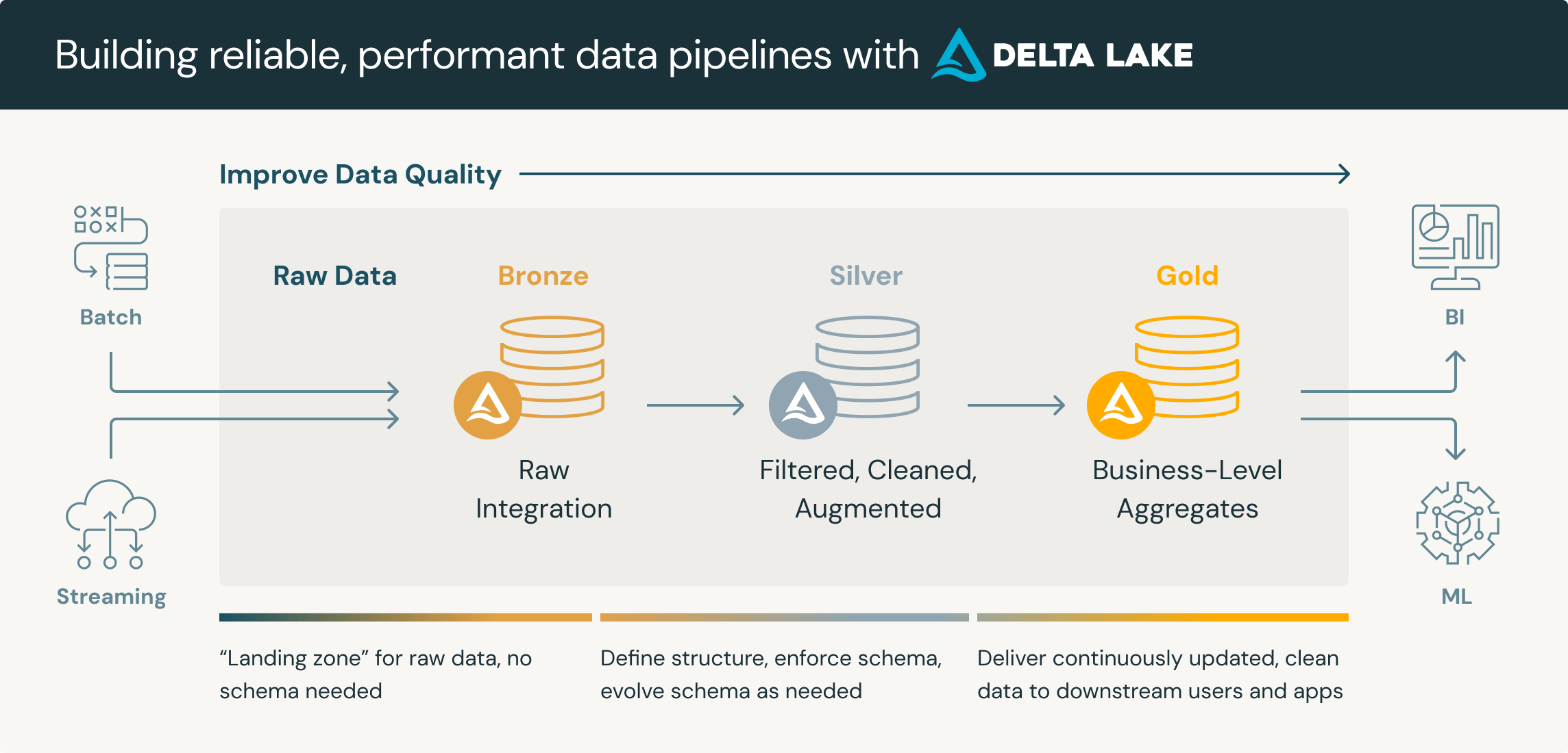
In case you use dbt for your data transformations, the chances are high that you’ve read about their suggested project setup of staging, intermediate and marts.
Where these fall short
In my view, the transformations themselves still need some structure, even if you follow the Bronze, Silver, Gold approach. But cramping 100+ transformations into the Gold-Layer or Modeling-Layer will eventually lead to an unmaintainable mess.
The suggested approach of structuring your transformations into 4 layers is neither unique nor new (e.g. here by WeWork), but indicates that others see the same need. Also, I don’t want to imply that the Staging-Layer or Silver-Zone don’t make sense, but they should be rather viewed as a complementary addition of structure.
So what are these 4 Layers about?

The general idea is that in each layer you can only work with data from the previous layer and - with the exception of Clean - the same layer. Also, resist the temptation of skip a layer as it most likely will backfire and cause more work later.
So let’s jump into what the layers are about in detail:
Clean
The Clean-Layer will be the solid foundation of your data transformations.
Numeric currency values loaded as STRING? Check.
Blank strings instead of NULL values sabotaging your COALESCE()? Check.
Useless test records included which will never be used? Check.
Parsing a JSON-payload into individual columns? Check.
Source- or ETL-Systems provide cryptic field-abbreviations? Check.
The “profile_id” which is actually a “customer_id”? Check.
…
The goal is to bring data types and field names into a standardized format so that you’re ready to apply more heavy logic. Once.
Every raw table you’ll use in your data pipeline must have exactly one cleaned table. This way, you’ll ensure that in case the table is used twice the steps are consistent and complete.
It’s comparable to the “staging”-part of the dbt approach. However, staging can mean different things depending on the context (see the raw-data landing zone from above? Or a “staging environment” …). The term “Clean” leaves less room for confusion in my opinion.
In case you use dbt, it’s suggested to have 1 folder per source system and mention the source system also in the filename:
clean/
  hubspot/
    clean_hubspot_contacts.sql
    clean_hubspot_deals.sql
    ...
  salesforce/
    clean_salesforce_accounts.sql
    clean_salesforce_opportunities.sql
    ...
This ensures sortability in your File Explorer as well as Database Editor.
Adding the table name of the cleaned table in there helps with finding if there is an existing clean-step for the specific table.
clean_{{ source system }}_{{ table_name }}Try to avoid any JOINs, business logic, or daisy chains in the Clean-Layer.
Focus on moving one raw table into one standardized table.
Prep
The Prep-Layer starts to transform data from application logic to valuable business logic.
You’re now allowed to join tables together and map values that are technically correct for the operational system, but provide no value for end users.
Operational systems only need to ensure correct operations. That’s why they rarely deliver analytics-ready information. A certain degree of logic on top always needs to be added to deliver proper value to business stakeholders.
Customer deduplication would be another common topic along with overwriting to which Account ID certain Transactions belong.
Here, you start to move away from the source system architecture of the Clean-Layer, and more toward the use-case-defined organization of models and tables.
If your transformations need a lot of space, you can break them down into smaller models, which are easier to digest and debug. Building a prep-model on top of a prep-model is generally OK.
Since you already filtered out useless data and did a lot of parsing and column renaming the business logic is a lot easier to understand.
What’s easier to pick up?
CASE
  WHEN PARSE_JSON(payload, r”transactions[0].date”)
     > PARSE_JSON(payload, r”creation_date”)
  THEN PARSE_JSON(payload, r”transactions[0].date”)
  ELSE ...
OR
CASE
  WHEN transaction_date > creation_date
  THEN transaction_date
  ELSE ...
Decide for yourself :)
For the table naming you want to indicate either what you’re building (e.g. “clean_googleanalytics_transactions” become “prep_marketing_order”) or what you’re doing if it’s a bigger transformation (“prep_dedup_customer”).
Did you notice the switch to singular names?
If you stick to - what’s considered the best practice of - naming the entities in their singular name (“order” instead of “orders”), do it already here.
Core
The Core-Layer should represent your Single Source of Truth (SSOT).
Regardless of the modeling approach, Dimensions & Facts vs Entities, you should have a single table per core asset defined here.
Customer belong to the VIP-Segment? You find it in Core.
Gross margin of a sales transaction? You find it in Core.
Order is dispatched? You find it in Core.
I’m not going too much into different modeling approaches - there will be dedicated content for that. But the idea is that you store the SSOT as granular as possible (often referred to as “atomic”) and maintain it in a single place (the Core-Layer).
The actual naming then depends on the modeling approach, too.
It might be “fct_sales”, “dim_product”, … in one approach or “product”, “sales” with an optional “core_” or “entity_” prefix in another one.
Do NOT daisy-chain core-models together. Move the logic to Prep instead.
You want to keep things as tidy and organized as these models might be exposed to Analysts later.
Mart
The Mart-Layer aims to provide ready-to-use datasets to technical- or business-oriented stakeholders or reports to cover the most common use cases.
But depending on your organizational setup and BI stack it might look very different.
There might be for example different marts exposed to business domains (Finance, Marketing, Product, …) in larger organizations. They might even add their own transformations on top if they have the resources and need for it.
For other, simpler settings, it’s simple pre-aggregations of the core-models.
Also, some BI tools prefer a classic star schema as input and resolve the relations between these tables internally. Then you might plug in your core-tables right away or just pre-aggregate them for increased performance.
Other BI tools prefer wider tables instead of joining tables. Then these denormalizations should happen in the Mart-Layer.
Another classic use case is the consolidation of information.
It might be impossible to join your new customers from the orders-table with the marketing_cost-table as this cost usually cannot be associated with a single customer. However, you might aggregate both tables along common attributes such as Date, Product, Country, and Marketing Channel to store them in aggregated, consolidated mart-tables.
Actuals vs Plan is another prime example of such a use case.
To keep logic DRY you might also re-use these consolidated mart-tables in other mart-tables. However long chains of mart-tables indicate, that some logic should be transferred upstream into the prep- and core-steps.
Transforming transaction data into a cohort shape to report accumulated lifetime value is also something that might turn out to be more complex and cumbersome in the BI tool itself. Shifting this logic and definition “to the left” into the Mart Layer saves you unnecessary computing in the BI Tool
and - hopefully - version-controlled logic in your Data Warehouse.
Summary
Using Bronze-Silver-Gold or Source-Staging-Modeling-Presentation Layers makes absolutely sense. However, too many times the transformations themselves lack the needed structure and maintainability.
Standardizing raw data first before correcting the application- with business logic is crucial. Separating your company’s core assets from specialized or abstracted marts is also important to keep a common understanding.
This approach addresses common challenges in data modeling by:
Promoting separation of concerns
Fostering consistent and maintainable data transformations
Providing flexibility for different organizational and tooling needs
If you then decide to use the suggested 4, just 3 or even 5 layers is up to you.
What’s your take on that? Did you have good results with anything different? And what topic you would like to see me write about in the future?
Super interesting approach, thanks for the sharing your thoughts! Just out of curiosity, how do you see architecture layering when end users (whether it'd be business users or a BI Tool) when the desire info is pre-aggregated state AND entity level break down. Would you say then best to provide access to both Core and Mart? Or this varying level of granularity should only be present in Mart? So perhaps another way of asking, should table with customer level purchases table and headline figures of purchases per cohort need to reside in Mart or one the first in Core and the latter in Mart?